Learning Objectives
Following this assignment students should be able to:
- start to combine multiple computing concepts to solve bigger problems
- start to debug errors in code
- use reproducible computing practices
Reading
Lecture Notes
Setup
install.packages(c('dplyr', 'ggplot2', 'readr'))
download.file("https://ndownloader.figshare.com/files/2292172",
  "surveys.csv")
download.file("https://ndownloader.figshare.com/files/3299474",
  "plots.csv")
download.file("https://ndownloader.figshare.com/files/3299483",
  "species.csv")
download.file("https://datacarpentry.org/semester-biology/data/mammal-size-data-clean.tsv",
  "mammal-size-data-clean.tsv")
Exercises
Bird Banding Multiple Vectors (20 pts)
The number of birds banded at a series of sampling sites has been counted by your field crew and entered into the following vector. Counts are entered in order and sites are numbered starting at one. There is also information on the number of trees at each site. Cut and paste the vector into your assignment and then answer the following questions by using code and printing the result to the screen.
number_of_birds <- c(28, 32, 1, 0, 10, 22, 30, NA, 145, 27, 36, 25, 9, 38, 21, 12, 122, 87, 36, 3, 0, 5, 55, 62, 98, 32, 900, 33, 14, 39, 56, 81, 29, 38, 1, 0, 143, 37, 98, 77, 92, 83, 34, 98, 40, 45, 51, 17, 22, 37, 48, NA, 91, 73, 54, 46, 102, 273, 600, 10, 11) number_of_trees <- c(10, 12, 2, 3, 10, 8, 19, 19, 14, 3, 4, 5, 8, 4, 8, 1, 12, 10, 3, 1, 2, 3, 5, 6, 8, 2, 90, 3, 4, 3, 6, 8, NA, 4, 0, 1, 14, 3, 10, NA, 9, 8, 4, 8, 4, 4, 5, 1, 2, 3, 5, 4, 10, 7, 5, 8, 10, 30, 26, 1, 6)- How many sites are there?
- How many birds were counted at the 26th site?
- What is the largest number of birds counted?
- What is the average number of birds seen at a site?
- What is the total number of trees counted across all of the sites?
- What is the smallest number of trees counted?
- Produce a vector with the number of birds counted on sites with at least 10 trees.
- Produce a vector with the number of trees counted on sites with at least 10 trees.
- Combine the
number_of_birdsandnumber_of_treesvectors into a dataframe that also includes a year column with the year 2012 in every row and site column containing the numbers 1 through 61.
Portal Data Review (20 pts)
If
surveys.csv,species.csv, andplots.csvare not available in your workspace download them:Load them into R using
read.csv().- Create a data frame with only data for the
species_idDO, with the columnsyear,month,day,species_id, andweight. - Create a data frame with only data for species IDs
PPandPBand for years starting in 1995, with the columnsyear,species_id, andhindfoot_length, with no null values forhindfoot_length. - Create a data frame with the average
hindfoot_lengthfor eachspecies_idin eachyearwith no null values. - Create a data frame with the
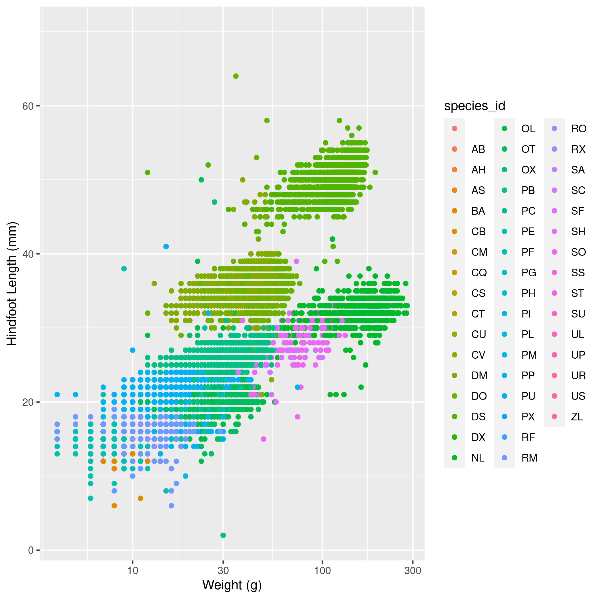
year,genus,species,weightandplot_typefor all cases where thegenusis"Dipodomys". - Make a scatter plot with
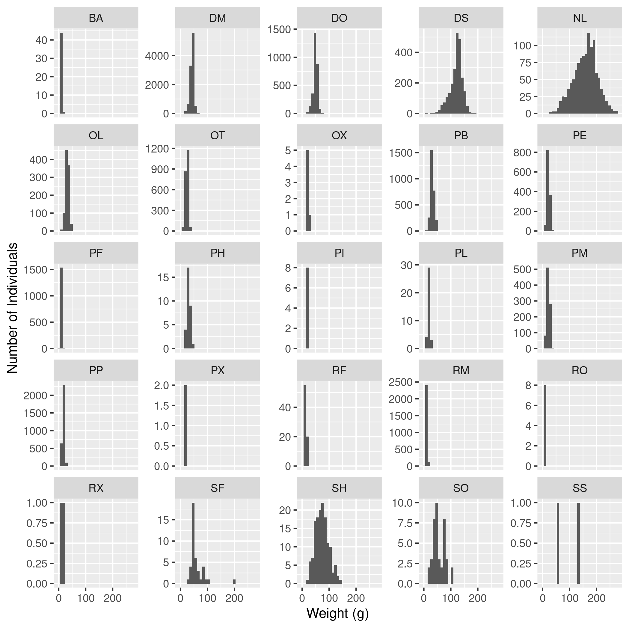
weighton the x-axis andhindfoot_lengthon the y-axis. Use alog10scale on the x-axis. Color the points byspecies_id. Include good axis labels. - Make a histogram of weights with a separate subplot for each
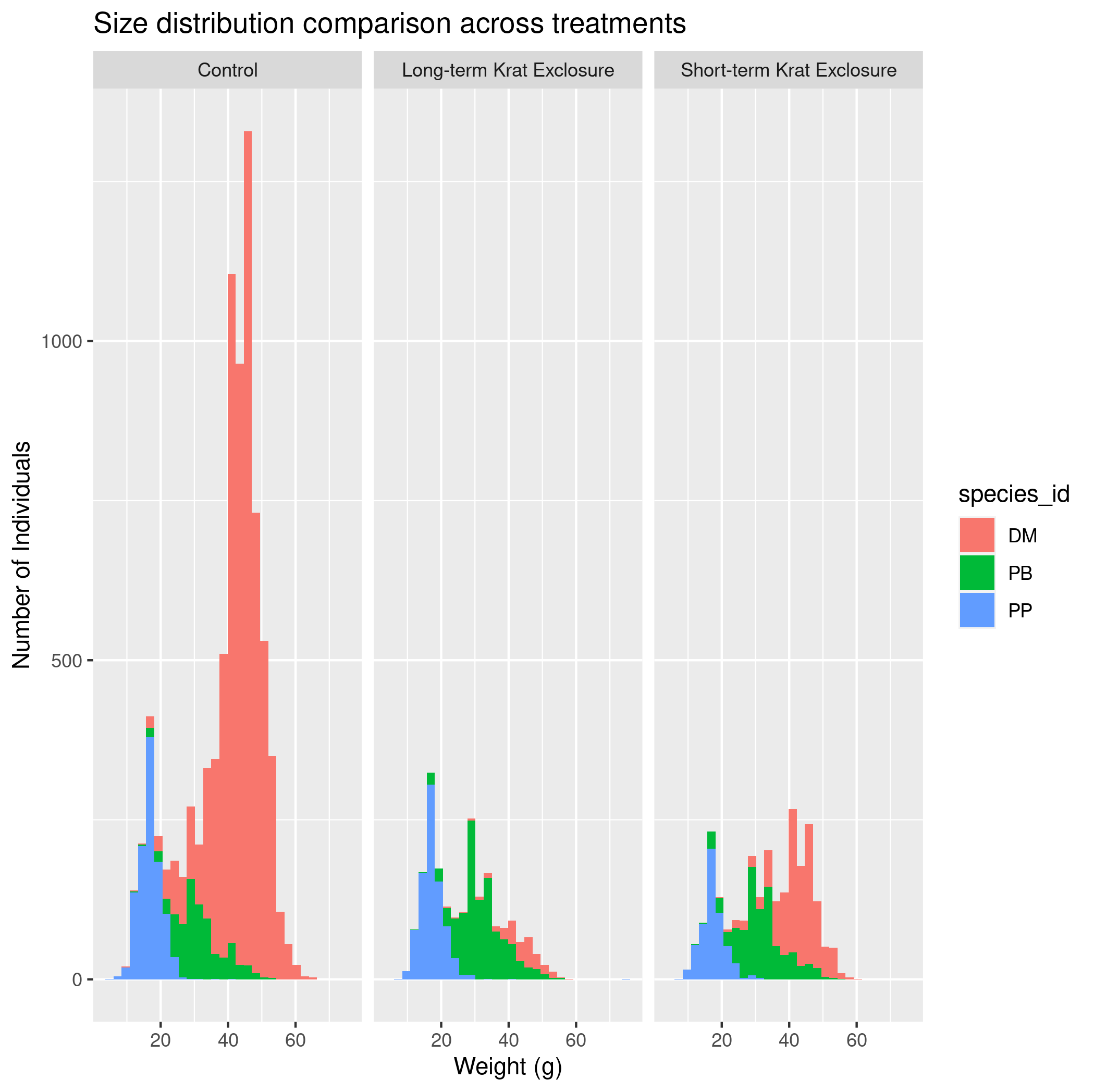
species_id. Do not include species with no weights. Set thescalesargument to"free_y"so that the y-axes can vary. Include good axis labels. - (Challenge) Make a plot with histograms of the weights of three species,
PP,PB, andDM, colored byspecies_id, with a different facet (i.e., subplot) for each of threeplot_type’sControl,Long-term Krat Exclosure, andShort-term Krat Exclosure. Include good axis labels and a title for the plot. Export the plot to apngfile.
- Create a data frame with only data for the
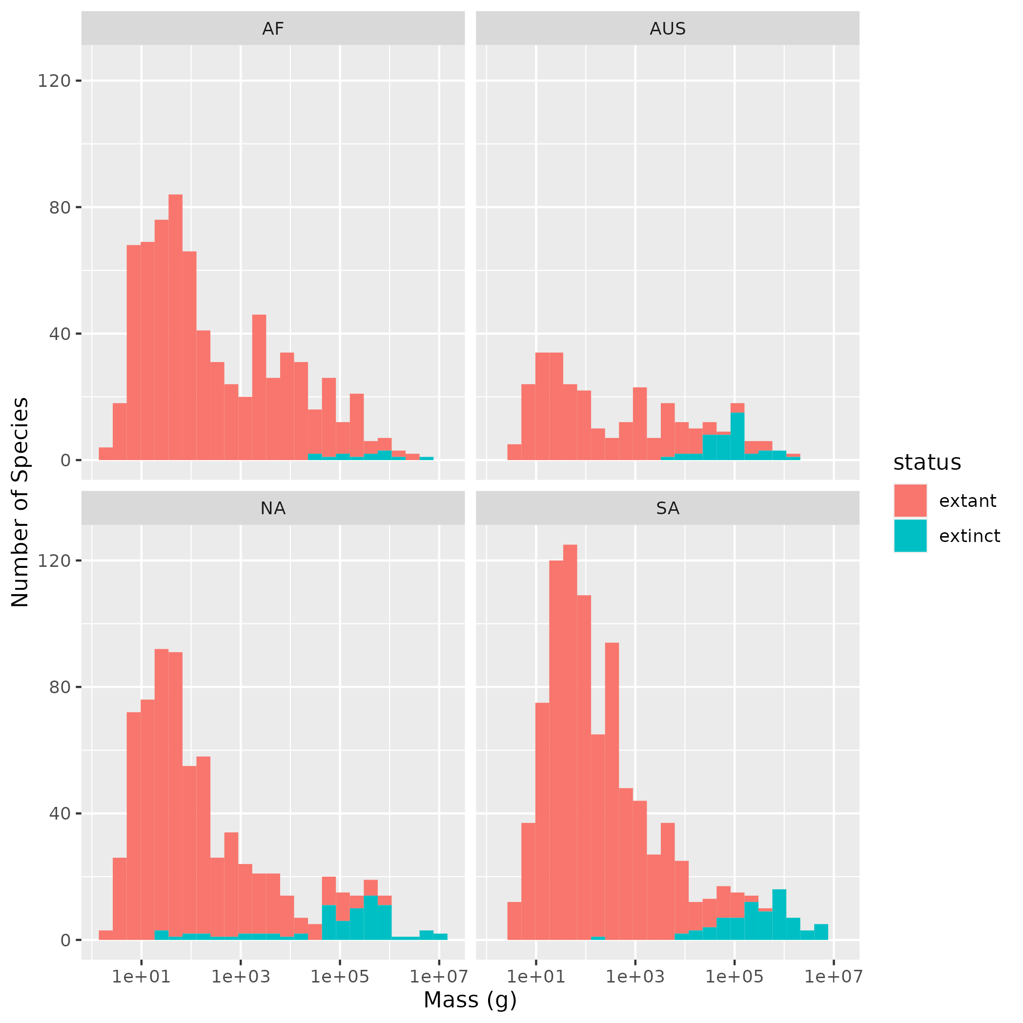
Megafaunal Extinction (60 pts)
There were a relatively large number of extinctions of mammalian species roughly 10,000 years ago. To help understand why these extinctions happened scientists are interested in understanding if there were differences in the size of the species that went extinct and those that did not. You are going to reproduce the three main figures from one of the major papers on this topic Lyons et al. 2004.
You will do this using a large dataset of mammalian body sizes that has data on the mass of recently extinct mammals as well as extant mammals (i.e., those that are still alive today).
- Import the data into R. As with most real world data there are a some things about the dataset that you’ll need to identify and address during the import process. Print out the structure of the resulting data frame.
- Create a plot showing histograms of masses for mammal species that are still
present and those that went extinct during the pleistocene (
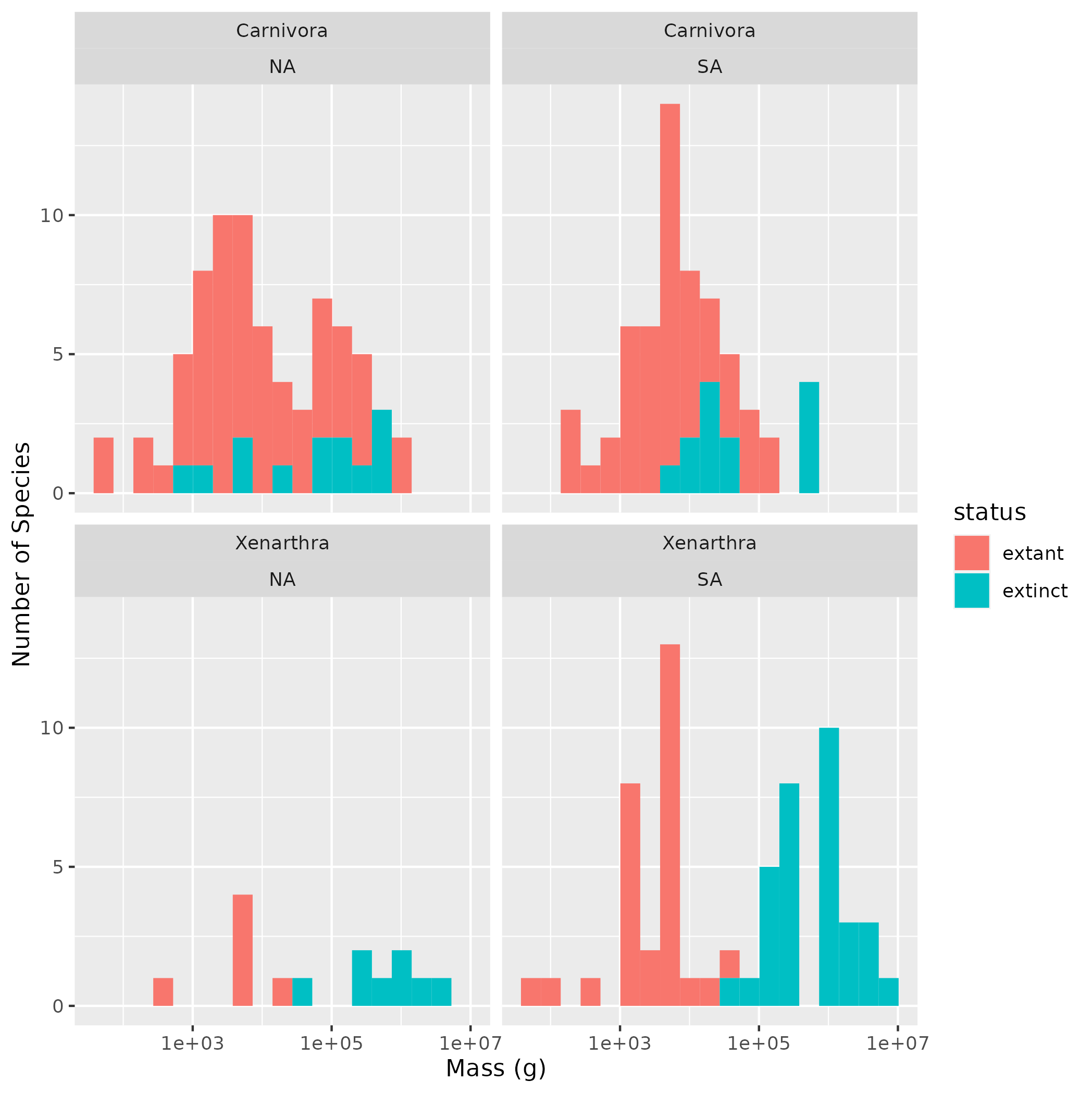
extantandextinctin thestatuscolumn). There should be one sub-plot for each continent and that sub-plot should show the histograms for both groups as a stacked histogram. To match the original analysis don’t include islands (InsularandOceanicin thecontinentcolumn) and or the continent labeledEA(becauseEAhad no species that went extinct in the pleistocene). Scale the x-axis logarithmically and use 25 bins to roughly match the original figure. Use good axis labels. - The 2nd figure in the original paper looks in more detail at two orders, Xenarthra and Carnivora, which showed extinctions in North and South America. Create a figure similar to the one in Part 2, but that shows 4 sub-plots, one for each order on each of the two continents. Still scale the x-axis logarithmically, but use 19 bins to roughly match the original figure.
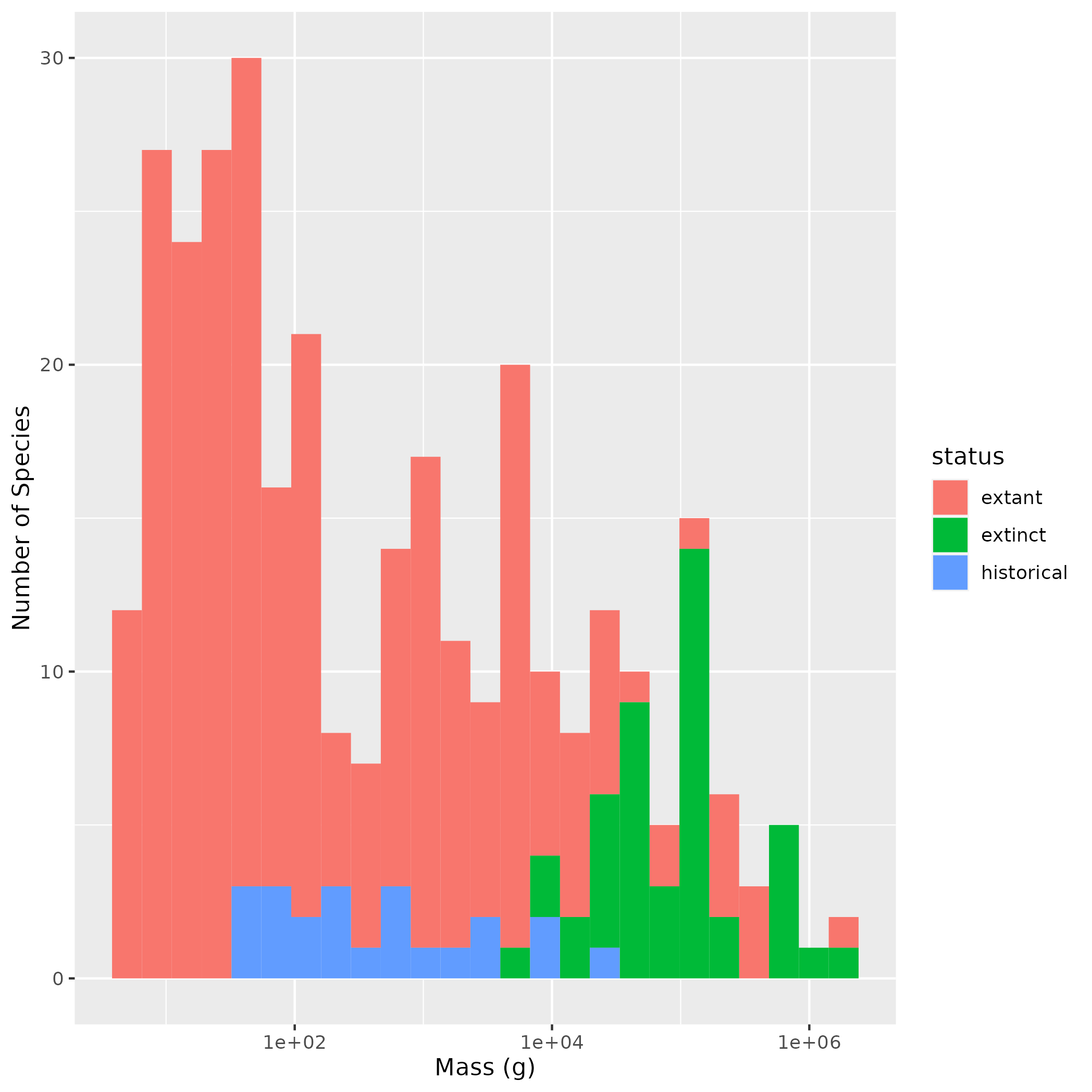
- The 3rd figure in the original paper explores Australia as a case study.
Australia is interesting because there is good data on both Pleistocene
extinctions (
extinctin thestatuscolumn) and more modern extinctions occurring over the last 300 years (historicalin thestatuscolumn). Make single stacked histogram that compares the sizes ofextinct,extant, andhistoricalstatuses. Scale the x-axis logarithmically and use 25 bins to roughly match the original figure. Use good axis labels. - (optional) Instead of excluding continent
EAby name in your analysis (in part 2), modify your code to determine from the data which continents had species that went extinct in the pleistocene and only include those continents.