Learning Objectives
Following this assignment students should be able to:
- import, view properties, and plot a
raster- perform simple
rastermath- extract points from a
rasterusing a shapefile- evaluate a time series of
raster
Reading
-
Topics
raster- Raster math
- Plotting spatial images
- Shapefile import
- Integrate
rasterandvectordata
-
Readings
-
Additional information
Lecture Notes
Exercises
Canopy Height from Space (30 pts)
The National Ecological Observatory Network has invested in high-resolution airborne imaging of their field sites. Elevation models generated from LiDAR can be used to map the topography and vegetation structure at the sites.
Check to see if there is a
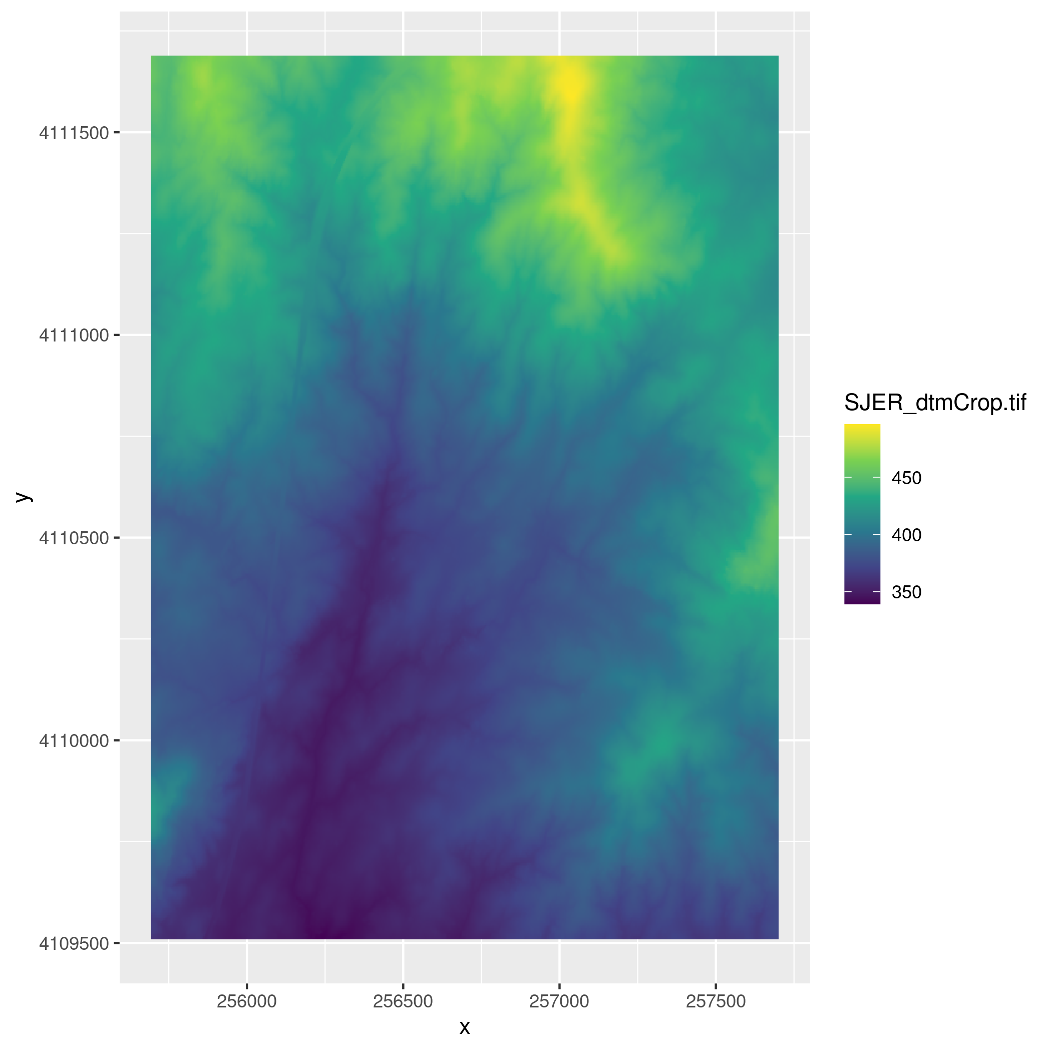
datadirectory in your workspace with anSJERsubdirectory in it. If not, Download the data and extract it into your working directory. TheSJERdirectory contains raster data for a digital terrain model (sjer_dtmcrop.tif) and a digital surface model (sjer_dsmcrop.tif), and vector data on plot locations (sjer_plots.shp) and the site boundary (sjer_boundar.shp) for the San Joaquin Experimental Range.- Map the digital terrain model for
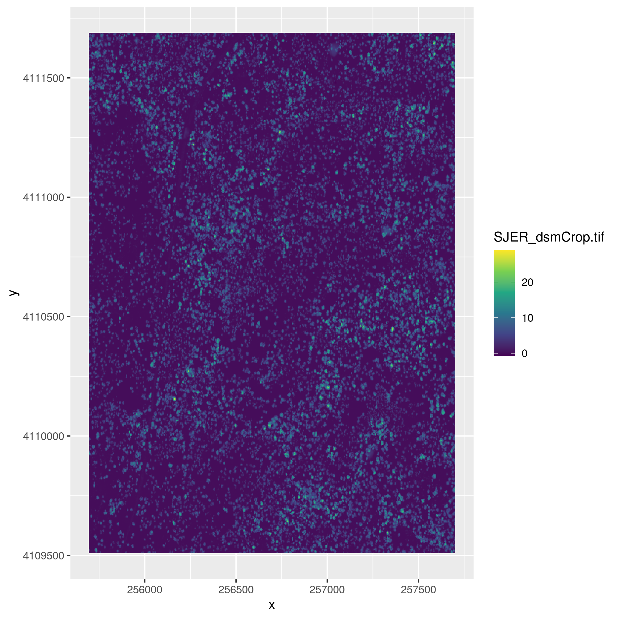
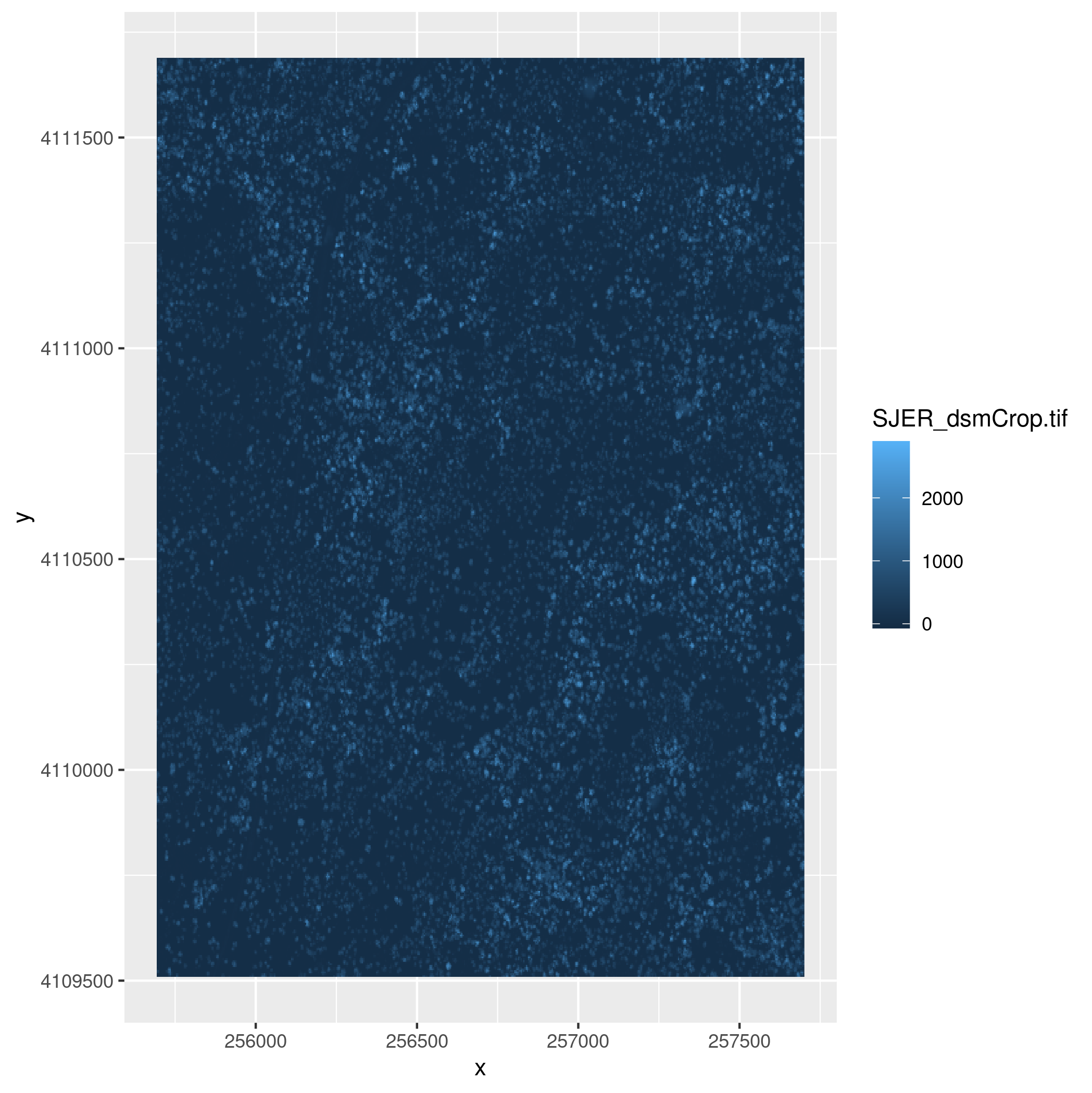
SJERusing theviridiscolor ramp. - Create and map the canopy height model for
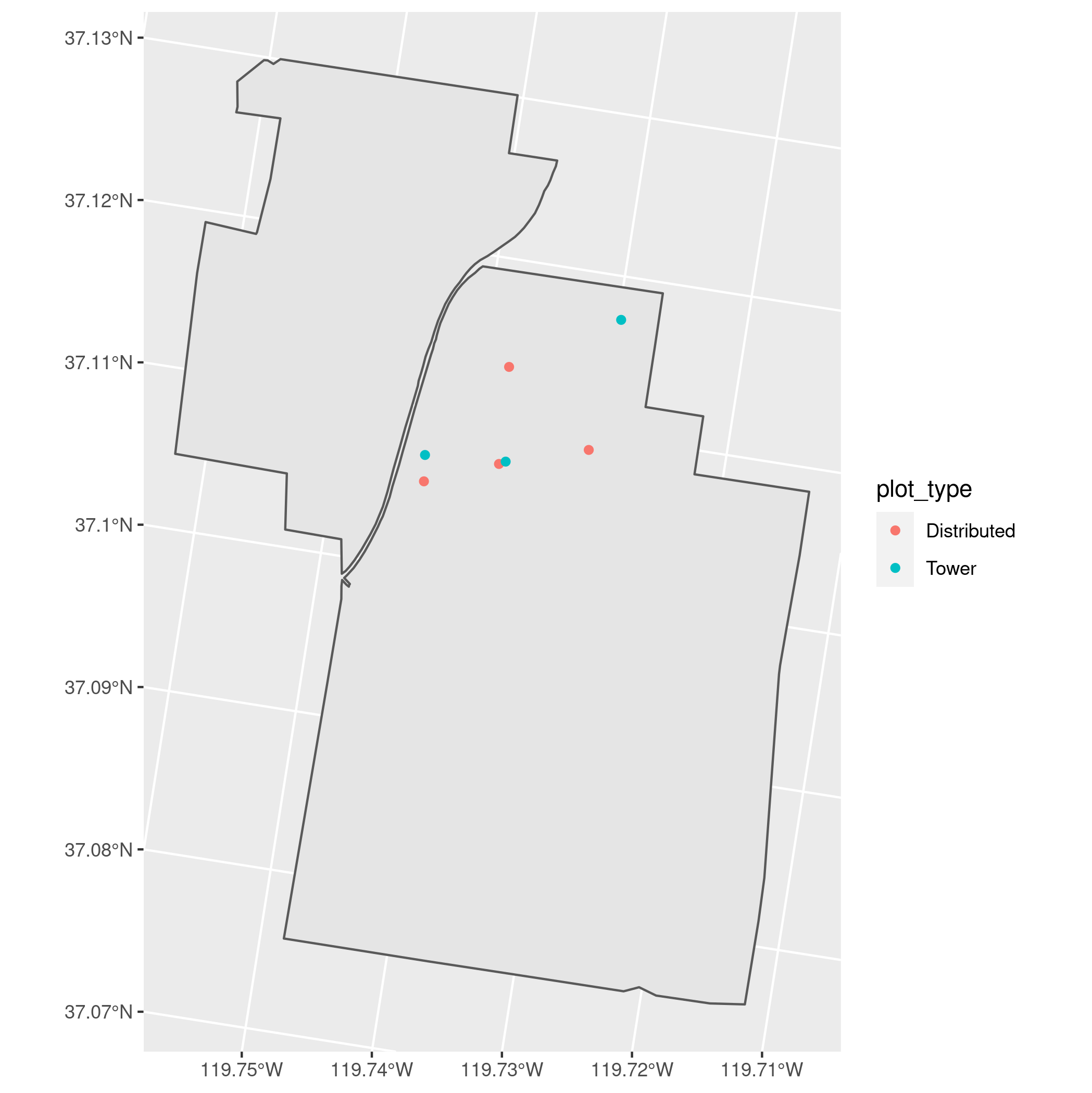
SJERusing theviridiscolor ramp. To do this subtract the values in the digital terrain model from the values in the digital surface model usingrastermath (chm = dsm - dtm). - Create a map that shows the
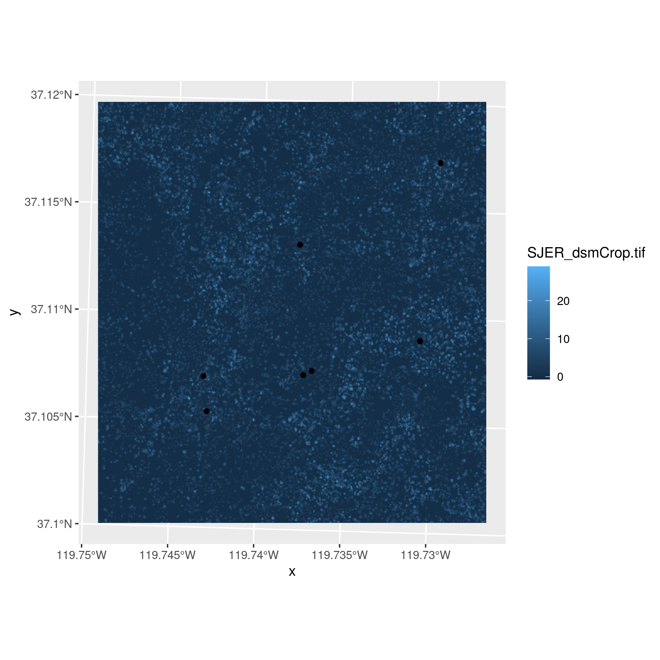
SJERboundary and the plot locations colored byplot_type. - Transform the plot data to have the same CRS as the CHM and create a map that shows the canopy height model from (3) with the plot locations on top.
- Extract the mean canopy heights at each plot location for
SJERand display the values. - Add the canopy height values from (5) to the spatial data frame you created for the plots and display the full data frame.
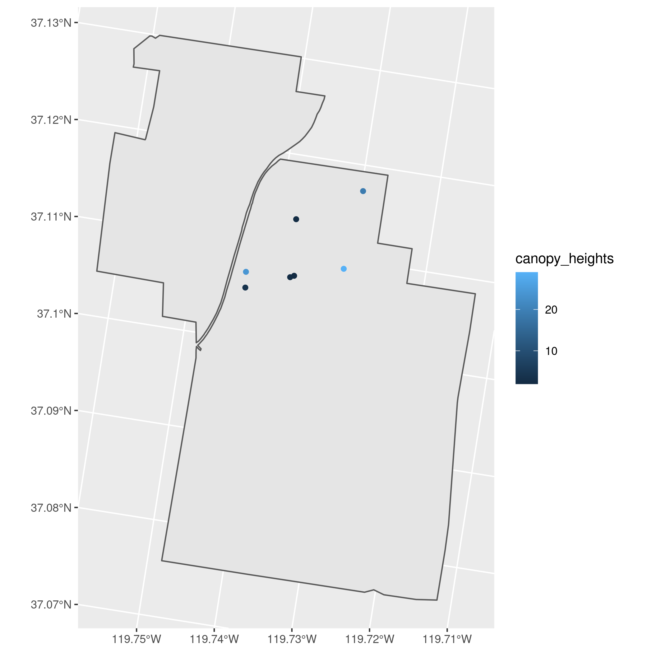
- Create a map that shows the
SJERboundary and the plot locations colored by the canopy height values. - Create a map that shows the canopy height model raster, but in
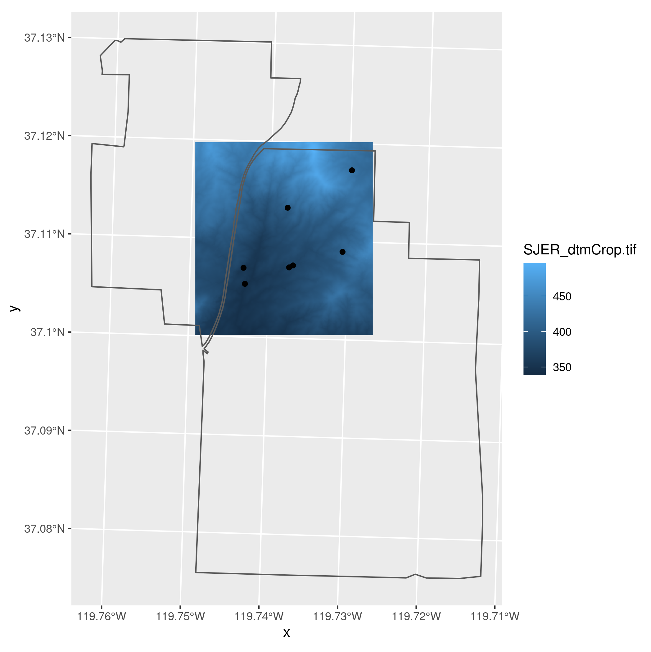
cmrather thanm(i.e., multiply the canopy height model by 100). - Create a map that shows the digital terrain model raster, the plot locations, and the
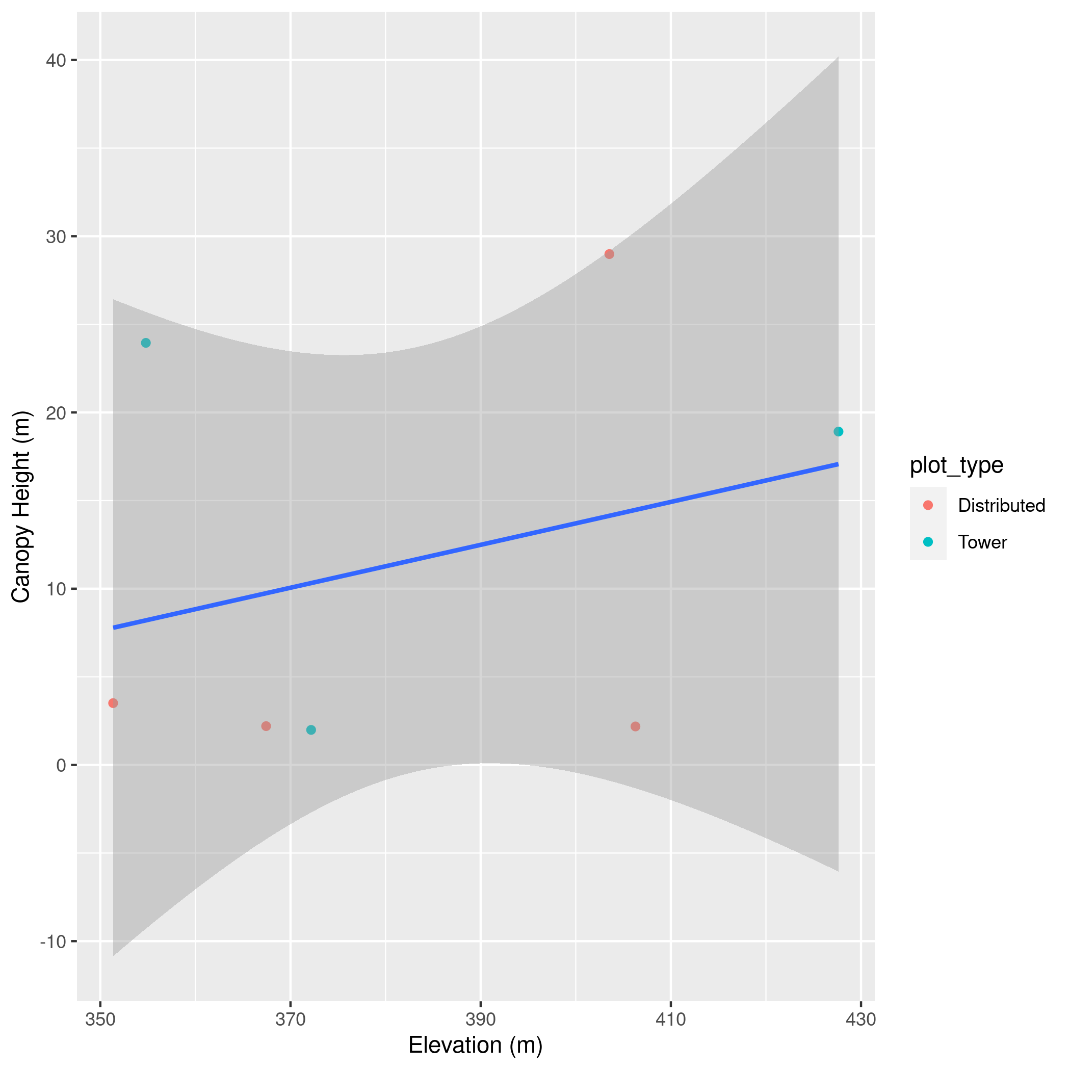
SJERboundary, using transparency as needed to allow all three layers to be seen. Remember all three layers will need to have the same CRS. - Conduct an analysis of the relationship between elevation and canopy height at the SJER plots. Start by extracting the mean elevations (i.e., the values from the digital terrain model) at each plot location for
SJERand adding them to the spatial plots data so that this data now includes both the elevations and the canopy heights. Then make a scatter plot showing the relationship between elevation and canopy height using this data. Color the points byplot_typeand fit a linear model through all of the points together (not separately byplot_type). Finally, usedplyrto calculate the average canopy height and average elevation for the two different plot types. Give the axes good labels.
- Map the digital terrain model for
Species Occurrences Map (40 pts)
A colleague of yours is working on a project on banner-tailed kangaroo rats (Dipodomys spectabilis) and is interested in what elevations these mice tend to occupy in the continental United States. You offer to help them out by getting some coordinates for specimens of this species and looking up the elevation of these coordinates.
Start by getting banner-tailed kangaroo rat occurrences from GBIF, the Global Biodiversity Information Facility, using the
spoccR package, which is designed to retrieve species occurrence data from various openly available data resources. Use the following code to do so:``` dipo_df = occ(query = "Dipodomys spectabilis", from = "gbif", limit = 1000, has_coords = TRUE) dipo_df = data.frame(dipo_df$gbif$data) ```- Clean up the data by:
- Filter the data to only include those specimens with
Dipodomys_spectabilis.basisOfRecordthat isPRESERVED_SPECIMENand aDipodomys_spectabilis.countryCodethat isUS - Remove points with values of
0forDipodomys_spectabilis.latitudeorDipodomys_spectabilis.longitude - Remove all of the columns from the dataset except
Dipodomys_spectabilis.latitudeandDipodomys_spectabilis.longitudeand rename these columns tolatitudeandlongitudeusingselect. You can rename while selecting columns using a format like this oneselect(new_column_name = old_column_name) - Use the
head()function to show the top few rows of this cleaned dataset
- Filter the data to only include those specimens with
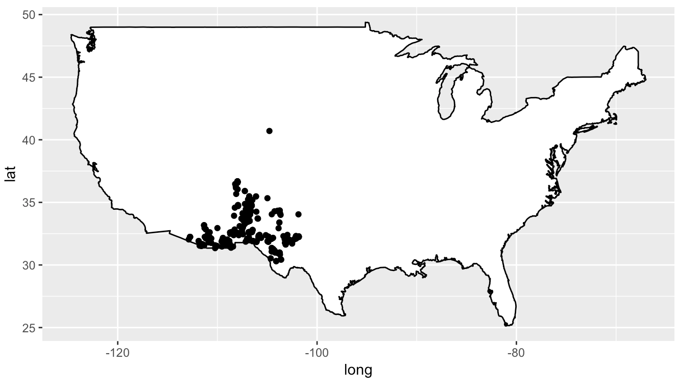
- Do the following to display the locations of these points on a map of the United States:
- Get data for a US map using
usmap = map_data("usa") - Plot it using
geom_polygon. In the aesthetic usegroup = groupto avoid weird lines cross your graph. Usefill = "white"andcolor = "black". - Plot the kangaroo rat locations
- Use
coord_quickmap()to automatically use a reasonable spatial projection
- Get data for a US map using
- Clean up the data by:
Species Occurrences Elevation Histogram (30 pts)
This is a follow up to Species Occurrences Map.
Now that you’ve mapped some species occurrence data you want to understand how environmental factors influnece the species distribution.
-
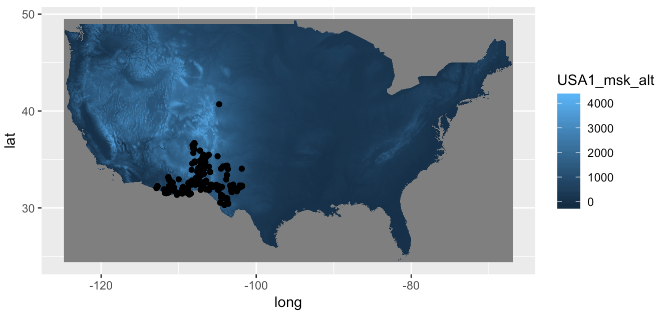
The
rasterpackage comes with some datasets, including one of global elevations, that can be retrieved with thegetDatafunction as follows:elevation = getData("alt", country = "US") elevation = elevation[[1]]Create a new version of the map from Species Occurrences Map that shows the elevation data as well. Plotting the elevation data may take a while because there are a lot of data points in the dataset. Pay attention to the order that the
geom_objects are plotted in. The name of the elevation variable isUSA1_msk_alt. If the website is down you can download a copy from the course site by downloading http://www.datacarpentry.org/semester-biology/data/wc10.zip and unzipping it into your home directory (/home/usernameon Mac and Linux,C:\Users\username\Documentson Windows) and using the commandelevation = getData("alt", country = "US", path = ".") -
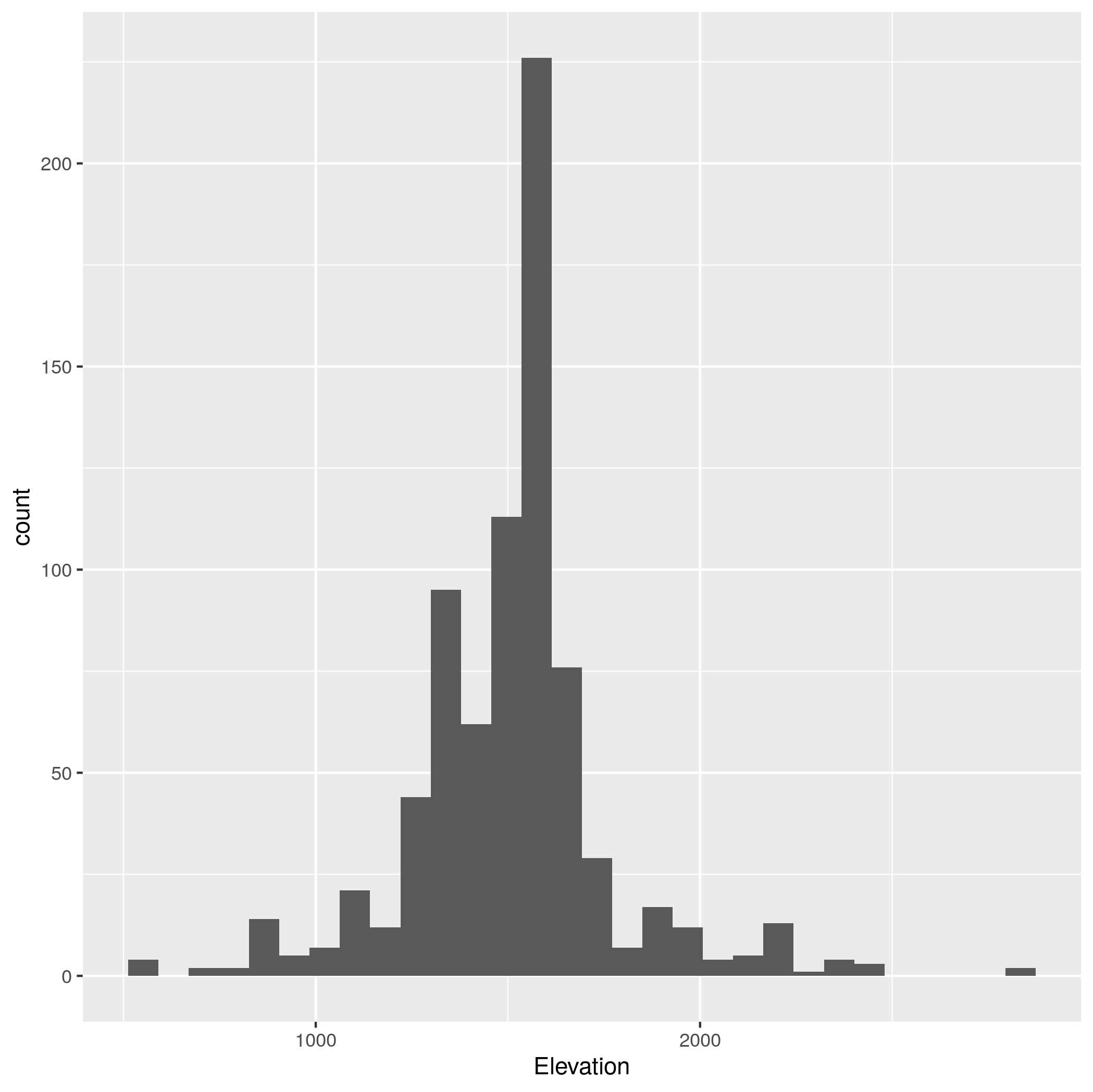
Turn the
dipo_dfdataframe from Species Occurrences Map into aSpatialPointsDataframe, making sure that its projection matches that of the elevation dataset, and extract the elevation values for all of the kangaroo rat occurrences. Turn this subset of elevation values into a dataframe and plot a histogram of the elevations. -
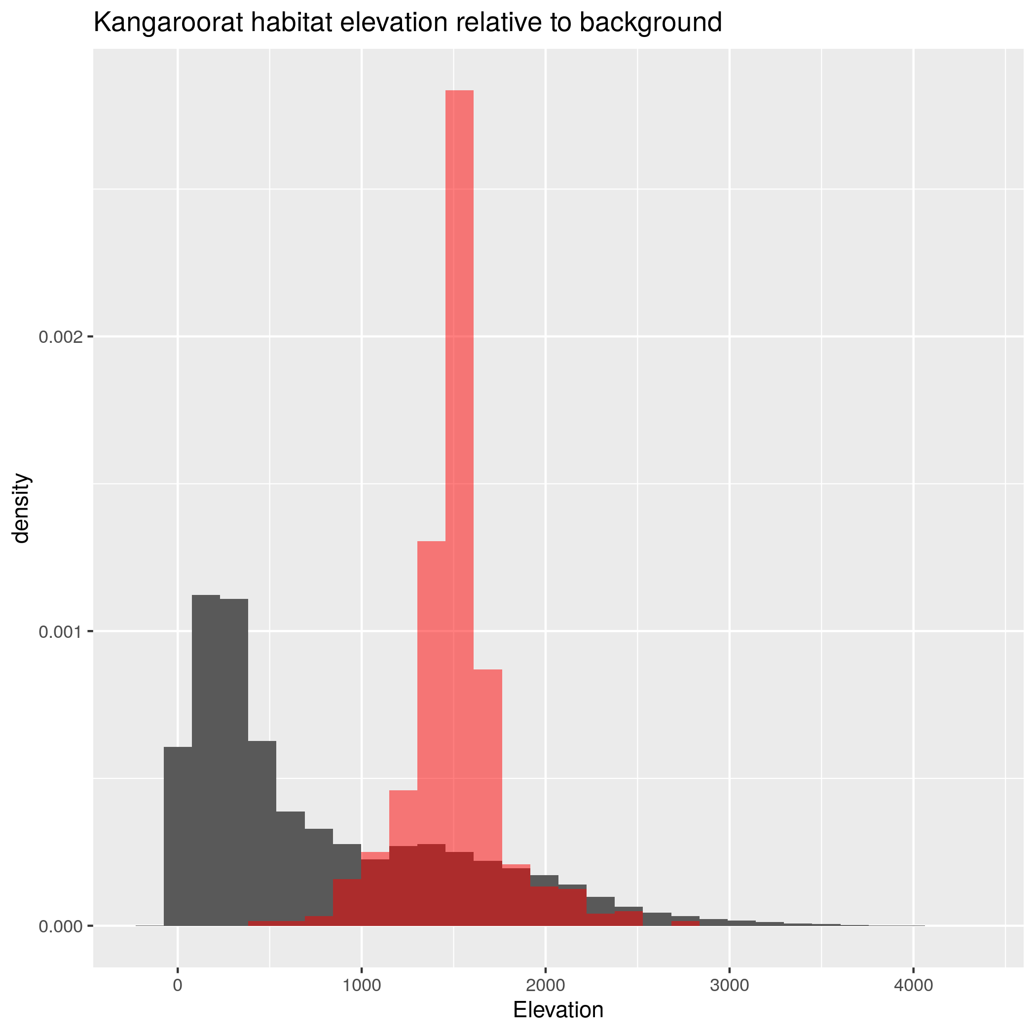
Part 2 showed us the elevations where banner-tailed kangaroo rats occur, but without context it’s hard to tell how important elevation is. Make a new graph that shows histograms for all elevations in the US in gray and the kangaroo rat elevations in red. Plot the kangaroo elevations on top of the full elevations and make them transparent so that you can see the overlap. To get the histograms on the same scale we need to plot the density of points instead of the total number of points. This can be done in
ggplotusing code like:ggplot() + geom_histogram(data = elevations, aes(x = USA1_msk_alt, y = ..density..))Lable the x axis elevation and add the title “Kangaroorat habitat elevation relative to background”.
-